Hello! Welcome to today’s lesson, in which I’ll show you how to identify winning positions in a game. This will help you to improve the strategy for your artificial intelligence in PyRat.
Winning strategies and positions
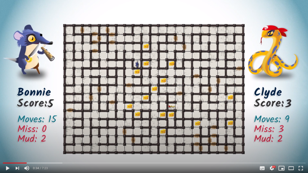
As you know, PyRat is a two-player game between a rat and a python, where each player must navigate a maze to find pieces of cheese hidden in the maze.
We say that a strategy for the rat is « winning » if the rat is sure to win the game, regardless of how the python decides to move. In other words, it’s a strategy such that, for any strategy of the opponent, the game is won.
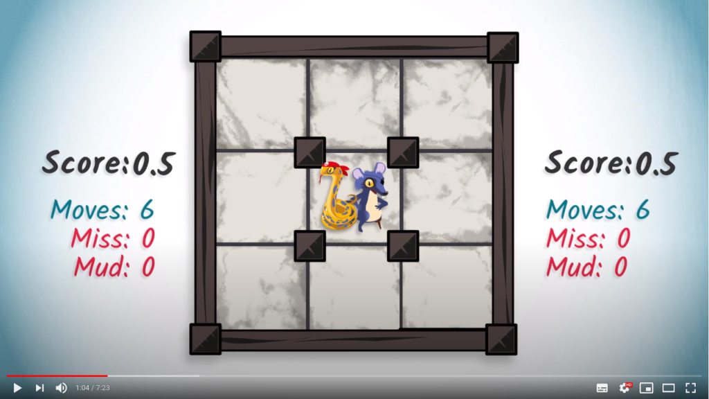
At the beginning of a game of PyRat, there is no winning strategy for any of the players, because the maze is symmetrical. Consequently, if both players choose the same strategy, then the result will be a tie.
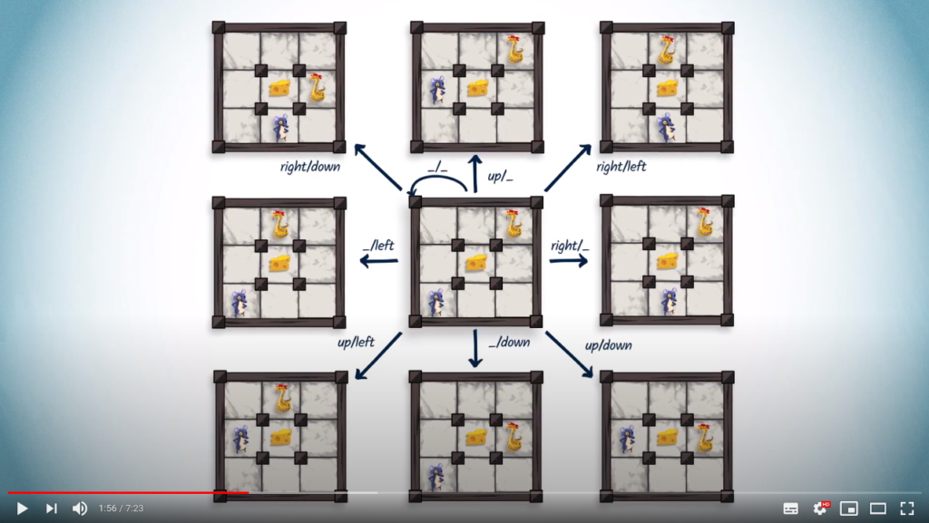
But once the game has started, and if the players at some point make different moves and break symmetry, the subsequent game will likely admit winning strategies for one of the players.
Determining if a winning strategy exists is a very complex computational problem. To do this, we need to consider two intertwined combinatorial factors, which are the possible strategies of the rat, and the possible strategies of the python. As a result, the number of possible games in PyRat is huge.
In practice, this means that computing winning strategies can only be performed when the variability of the game is reduced, such as when there are just a few pieces of cheese left in the maze.
Let’s now return to the concept of arena. You probably remember from the previous lesson that the arena is a graph where each vertex summarizes the actual state of the game.
A vertex in the arena is a winning position for a player if, starting from that vertex, the player has a winning strategy.
Of course, a vertex cannot be winning for both players. If this were the case, it would mean that both players have a strategy that wins against any strategy of the opponent. This would imply that when they both play with their winning strategies they both win, which is not possible. So a vertex can only be winning for one player.
Computing winning strategies
So now let’s see how to compute winning strategies. Ready?
If you’re at a given vertex in the arena, to find the best move, the one that keeps you in the winning region of the arena, you have to take into account all possible subsequent choices of the opponent. In a game like PyRat, the number of such combinations is probably too big to be processed.
Imagine a game of PyRat that is limited to 2000 decisions for each player. At each step, both players choose a direction to move in. At the very minimum, each player has one of two choices to make – to move or not to move. In that case, the number of possible games is at least , which is huge.
A better approach involves storing partial knowledge about winning strategies and positions. This type of approach is called « dynamic programming ».
It’s possible to characterize the state of a game by the position of the rat, the position of the python, the locations of remaining pieces of cheese, and the score of each player.
Again, imagine a PyRat instance in which the maze contains 15×11 cells, that is, 165 cells, and let’s say that there are 7 pieces of cheese. Note that we do not need to retain the actual locations of the pieces of cheese, since they will not move during the game, but we only need to retain which ones have been eaten and which ones are still in the maze. So in this example, there are 2 possible configurations for each of the 7 pieces of cheese, which makes a total of possible configurations. Also, there are 165 possible positions for each player. Regarding the scores, we only need to store the score of one player, because this, along with the remaining pieces of cheese, can be used to retrieve the score of the other player. So there are 5 possible scores for one player, between 0 and 4. Finally, there’s a maximum of million vertices in the arena.
Remember that the vertices in the arena represent game configurations.
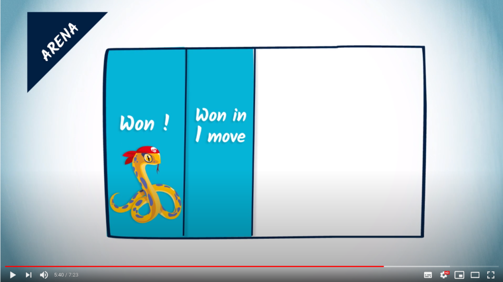
So one way to compute winning strategies starts by first identifying vertices in the arena, here represented by the rectangle, in which the game is already won for a player. In the previous example, this comes down to determining all vertices where one of the players, for example the python, has a score of 4.
Now we can try to identify other vertices of the arena where one of the players is ensured to win.
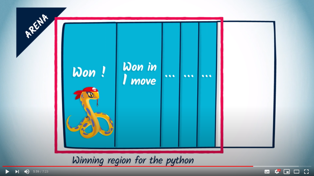
For example, these are all the vertices from which the player can choose a move such that no matter what the choice of the opponent is, the player reaches a vertex in the arena already identified to be a winning one.
By repeating this process until no more vertex can be added to the list of winning ones, we are actually building a winning strategy for the player and at the same time computing his winning region of the arena.
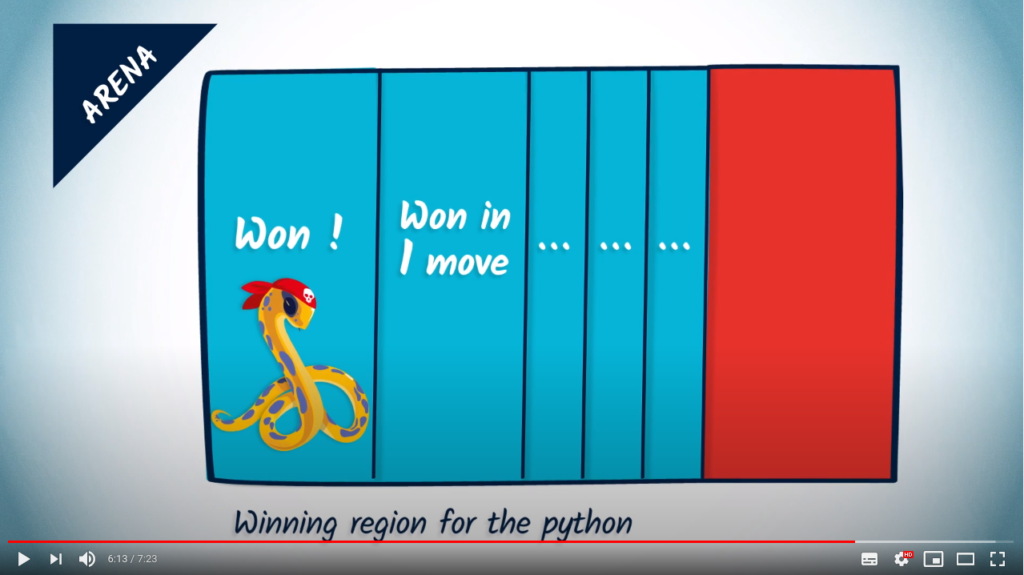
In the remaining region of the arena, whatever the python does, the rat can always move in a way that avoids entering the blue region of the arena. As a consequence, there is no winning strategy for the python in the red region.
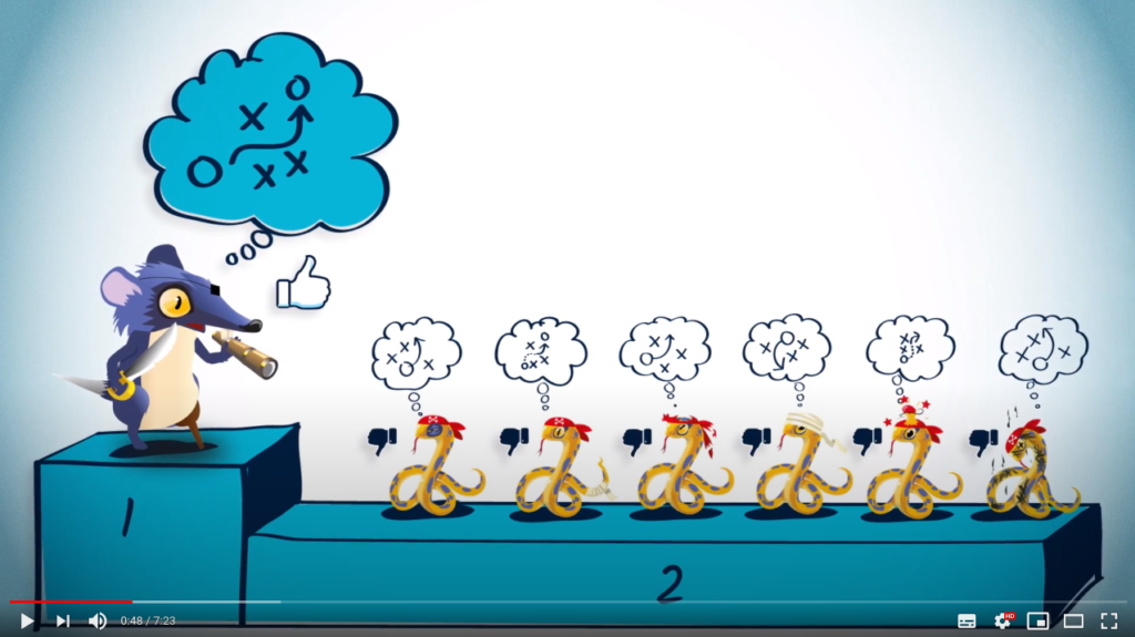
You should note that that this way of building a winning strategy can only be computed for a small maze with a limited number of pieces of cheese, and isn’t really feasible for large mazes. When it comes to large mazes, a better approach would involve making assumptions about the opponent’s decisions, which would reduce the combinatorial factors.
Concluding words
This finishes today’s lesson. You’ve learned how winning strategies can be generated, but also that, for larger games and for some computational issues, it might be necessary to take the opponent’s strategy into account.
It’s now up to you to implement all this in your AI in PyRat!
Sadly, this video was the last one in this MOOC. I have really enjoyed exploring the topics of this course with you! Vincent, Nicolas and I hope that you’ve learned many fascinating things on algorithms, and that your AI will be clever enough to beat many opponents.
May the cheese be with you!
The maximin algorithm
In game theory (more precisely in complete information, zero-sum games), the maximin algorithm aims at finding the best move to make at each step, assuming the opponent will play optimally. The goal for the opponent is therefore to minimize our gain, while ours is to maximize it.
Concretely, the main idea of the algorithm is to start from the leaves of the tree of solutions, and to give a score to each of these leaves, corresponding to the gain it provides us.
Then, we will go up the tree until we reach the root, by alternating minimizations of the scores, and maximizations. This alternance models the choices of either the player, or the opponent.
Example
Let us describe what happens on an example, taken from the French Wikipedia page on the Minimax algorithm (minimax is just the symmetric problem of maximin in which we want to minimize some loss function rather than maximizing a gain):
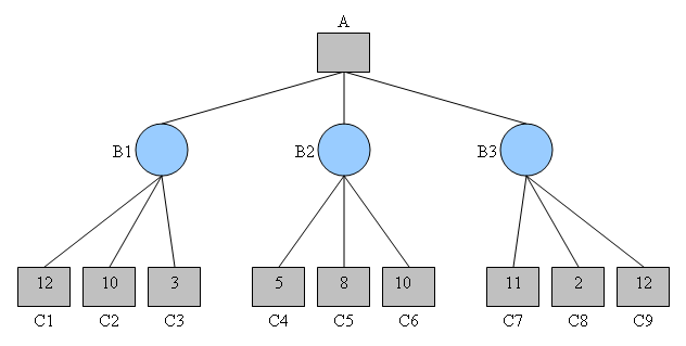
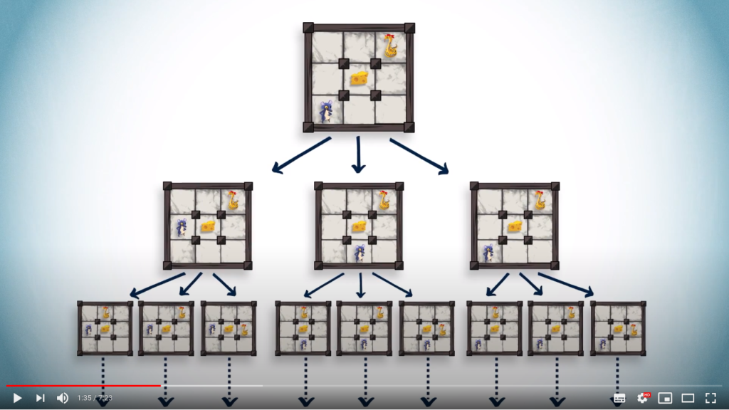
Possible executions of a game.
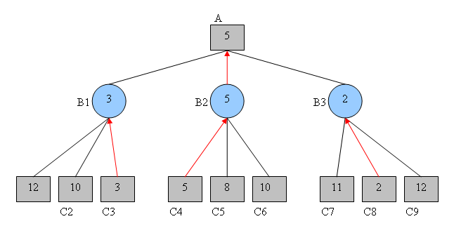
Here, we have a tree of possible executions of a game, in which depths modeled with squares indicate our turn to play, and circles indicate the opponent’s turn.
For each circle node, the opponent will try to minimize our gain, by choosing to perform the action that leads to the minimum gain for us. Therefore, the minimax algorithm will assume the following choices:
The opponent will minimize our gain.
What it now means is that, if I reach the state of the game B1, the opponent will play so that our total gain is 3, obtained from state C3. If we make the game go to state B2, our opponent can play so that gain is 5 by enforcing state C4. Finally, if we play to reach situation B3, the opponent can play so that gain is 2 by enforcing state C8.
The optimal choice for us is therefore to maximize the gain, and to play so that we reach state B2. Making this choice, the best gain one can expect when facing an optimal opponent is 5:
We will maximize our gain.
The minimax algorithm consists in alternating these steps of minimizations and maximizations, in order to maximize the gain we would ultimately expect when making a decision.
It is important to notice that the maximin algorithm will not return the sequence of plays that lead to the highest achievable gain (which in the example above would be C9 with a gain of 12), but the least worst sequence of play, i.e., the one that realistically leads to our best gain.
To conclude, notice that here we alternate decisions between players, which implies they take their decisions in turn. Still, there exist equivalent results for simultaneous games such as PyRat.

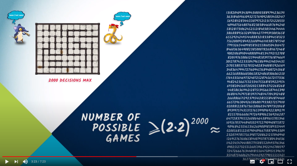
 , which is huge.
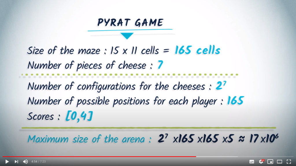
 possible configurations. Also, there are 165 possible positions for each player. Regarding the scores, we only need to store the score of one player, because this, along with the remaining pieces of cheese, can be used to retrieve the score of the other player. So there are 5 possible scores for one player, between 0 and 4. Finally, there’s a maximum of
  million vertices in the arena.