Hi, and welcome to this lesson on Dijkstra’s algorithm!
This week, we’re going to talk about shortest paths in weighted graphs. The graph traversal algorithms that we’ve already looked at in the previous lesson can’t be directly applied to find shortest paths in weighted graphs.
Weighted graphs
To illustrate why the graph traversal algorithms already presented do not necessarily work for weighted graphs, consider the following toy graph.
Here, a breadth-first search, BFS, starting from vertex , will not produce a spanning tree of shortest paths. For example, the actual shortest path from to is , , where the path found using a BFS is .
This is because a BFS favors a smaller number of hops from the initial vertex, regardless of the weights.
Dijkstra’s algorithm
Dijkstra’s algorithm is a modification of the BFS that allows us to find shortest paths, even in the presence of weights, if those are non-negative.
A quick note about weights. So far in this MOOC, we’ve only considered weights that are non-negative. In some cases it might be meaningful to add negative weights.
For example, imagine a taxi driver that can travel between cities. Sometimes he earns money because he has a client and sometimes he loses money because he travels alone. We could thus consider a graph whose vertices represent cities and edges are weighted by the cost of the corresponding travel. Some weights would then be positive and others negative.
Let’s get back to graphs with non-negative weights. The simplest way to describe Dijkstra’s algorithm is to imagine the starting vertex as a tap from which water is pouring out. The water will progress along the vertices and traverse the graph with a speed inversely proportional to the edge weights, so it’s going to reach the closest vertices first.
In other words, the Dijkstra’s algorithm is a traversal algorithm in which vertices are visited by increasing distance from the initial vertex.
At each step, the Dijkstra algorithm stores two kinds of information: 1) which vertices have already been explored, and 2) an approximation of distances from to all other vertices in the graph.
The Dijkstra algorithm repeats two steps. In step 1, it selects an unexplored vertex that is at a minimum distance from . In step 2, it updates the distances from to the other vertices of the graph, using information about and its neighbors.
Note that the algorithm always yields a spanning tree of minimum paths in the graph, provided weights are non-negative. We’re not going to prove this result here, but it’s not so hard to do a very nice exercise if you’d like to go a little deeper into the concepts described in this lesson.
Let’s describe more precisely how the Dijkstra algorithm works using the following example. We’re going to build a minimum spanning tree starting from vertex in this graph.
So, we initialize two data structures: first, the set of explored vertices, which are initially empty, and second, the array of distances from to the other vertices in the graph, initialized to everywhere but , where we insert a 0.
The first step is to select a non-explored vertex that is at minimum distance from the starting vertex. Here, we select as our starting vertex and add it to the set of explored vertices.
The second step is to update the distances taking into account the selected vertex , and its neighbors. Here, has two neighbors: and . Reaching them in one hop from costs 5 and 3, respectively. So we update our distances from by saying that is at distance 5 and is at distance 3. Note that the length of a shortest path from to is actually 4, but that we can’t tell that yet given the results from the algorithm alone.
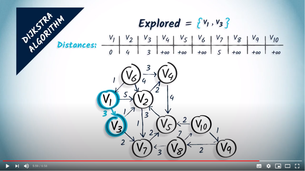
Let’s now start a new iteration of the algorithm. In the first step, we select an unexplored vertex at a minimum distance from . Here, we choose , which is at distance 3. We add it to the set of explored vertices.
In the second step, we look at the neighbors of , which are and , with corresponding weights of 1 and 2. So, if we want to reach by going through one hop before, we have a total cost of 3, which is the cost to go to , plus 1, which is the cost of doing one hop from to . This is better than the previous distance we estimated for , so we modify the distances accordingly. As far as is concerned, we now have an estimated distance of 3, the cost of going to plus 2 which is the cost of one hop from to .
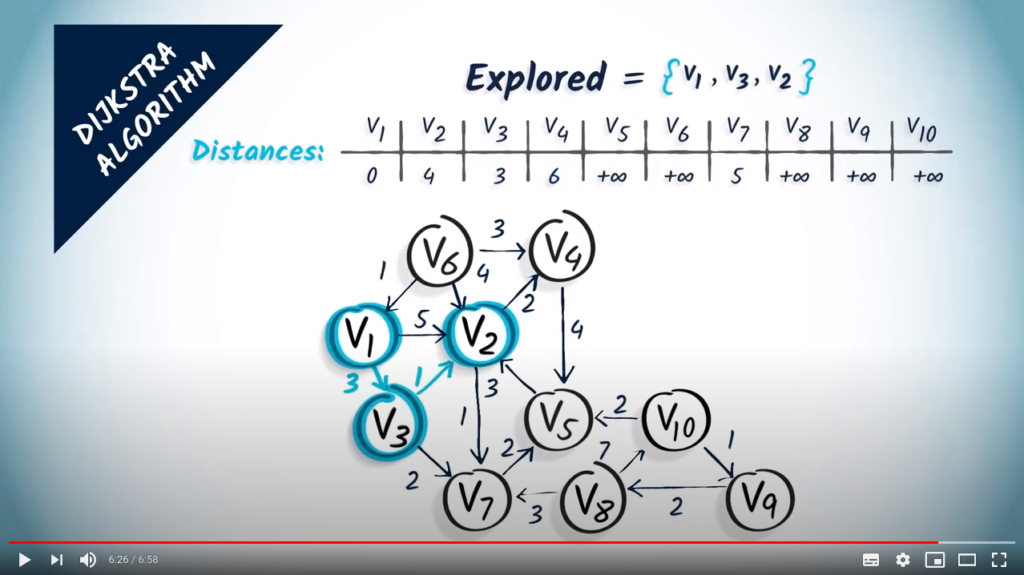
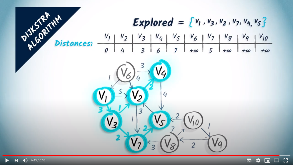
A new iteration begins. Now we select the next unexplored vertex with the smallest distance, which is . We add it to the set of explored vertices.
The vertex has two neighbors, and . The vertex is estimated to be at distance , and at distance . So we update the distance to . As far as is concerned, the newfound distance is not better than the old one, so it has no effect.
A new iteration begins. We select at distance 5 and add it to the list of explored vertices. And so on…
Finally we obtain the following spanning tree.
Concluding words
That’s all for this lesson! Next we will see how to implement Dijkstra’s algorithm by using min-heaps.
Properties of Dijkstra’s algorithm
Termination & correctness
We want to show that Dijkstra’s algorithm ends and is correct if all weights in the graph are strictly positive.
The proof of correction and termination for Dijkstra’s algorithm is more complicated than those we have already seen for more simple traversal algorithms. We’re going to do both at the same time.
Let’s assume a priority queue (here, a min-heap) for which all operations terminate and are correct. If the notion of min-heap does not ring you a bell, you should read this article first.
For the proof, we will proceed by recurrence with the following property: all the vertices that have been removed from the priority queue are such that their distances from the initial vertex have been calculated and recorded, and the remaining vertices, if any, are all at a greater distance.
We notice trivially that this statement is true at the first pass in the loop, when we remove the initial vertex.
Let us now assume this statement to be true at some point during the execution of the algorithm. There are two cases:
Either the priority queue is empty, in which case the algorithm stops and the property remains true;
Or a new couple (current node, distance) is extracted from the priority queue.
We want to show that the extracted distance is the distance of a shortest path from the initial vertex to the current vertex.
We must note that this is already the length of a path in the graph. Indeed, the distance was updated at a time when another vertex was previously removed. By hypothesis of recurrence, this corresponded to a shortest path, and the vertices being neighbors, we obtain a quantity corresponding to the length of a path.
Then, it is necessarily the length of a shortest path. Indeed, let us consider a shortest path in the graph from the initial vertex to the current vertex and let us denote previous vertex the one immediately before the current vertex along this path. By definition of the shortest path, the subpath extracted from the initial vertex to the previous vertex is a shortest path to that vertex. This subpath is strictly shorter because it contains one edge less (and the edges have strictly positive weights). In the event of a recurrence, the previous vertex has already been removed from the priority queue. And therefore the distance to the current vertex was either set to its minimum value at that time, or was already there before (it could not be less since it is the length of a path in the graph).
By recurrence we conclude that the property is true at any stage of the algorithm.
To finish proving the correction and at the same time have the termination, we still have to show that:
Each vertex can only be removed once from the priority queue;
Any reachable vertex is removed at least once.
For 1., this is directly deduced from the increase in distances proven in the previous recurrence.
For 2., we notice that any reachable vertex admits a shortest path, and we proceed by recurrence along this path.
Complexity
The algorithm complexity depends heavily on the priority queue used. We can show that the complexity can be attained when using an adapted structure.
In the particular case of the maze we work on in PyRat, each vertex has at most 4 neighbors. Therefore, we obtain a complexity of , since . As this complexity is less than quadratic, it is quite reasonable for our problem.
To go further
Fibonacci heap: a data structure to improve execution time of Dijkstra’s algorithm.

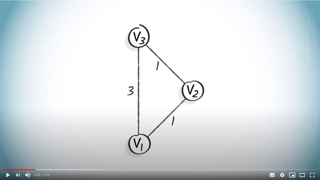
 , will not produce a spanning tree of shortest paths. For example, the actual shortest path from
  is
is  ,
,  , where the path found using a BFS is
  .
.


 that is at a minimum distance from
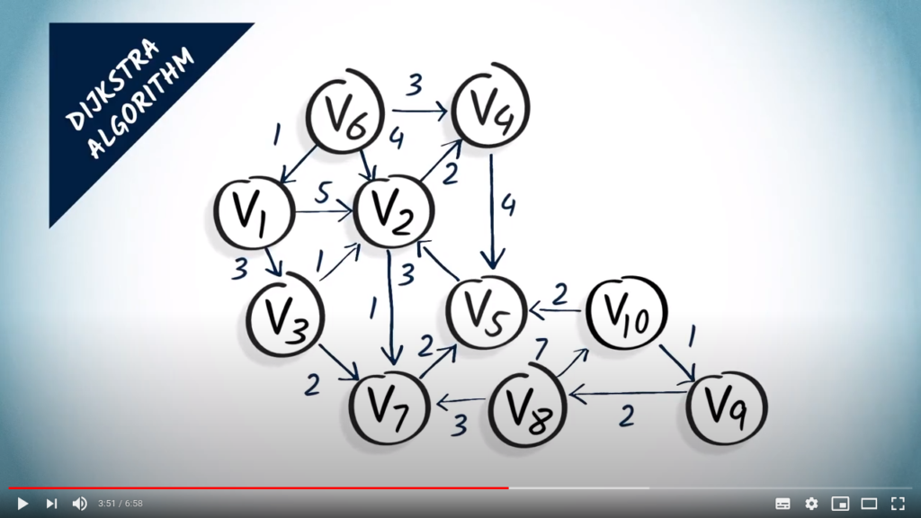
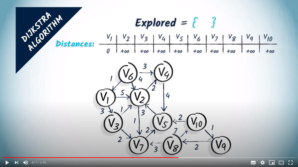
 everywhere but
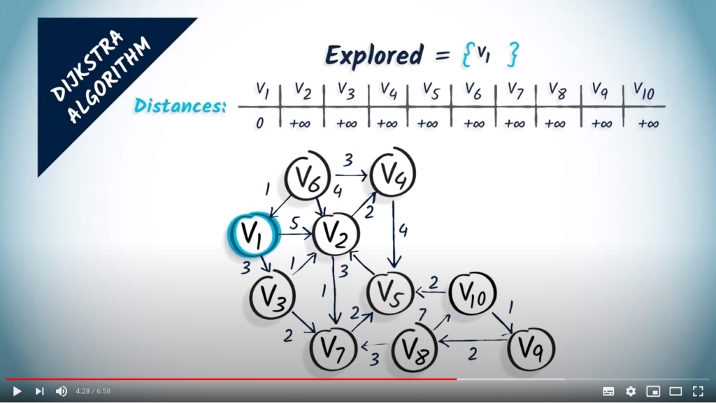

 and
and 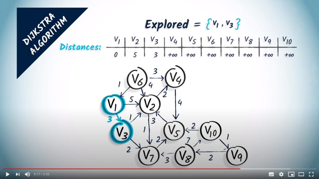
 , with corresponding weights of 1 and 2. So, if we want to reach
 and
and  , and
, and  . So we update the distance to
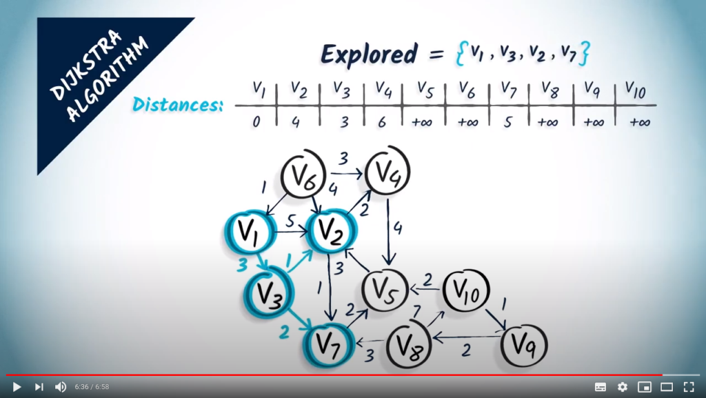
 can be attained when using an adapted structure.
 , since
  . As this complexity is less than quadratic, it is quite reasonable for our problem.