Hi! And welcome to this lesson about graph traversal.
Finding the exit of a maze requires us to traverse part of the maze. Graph traversal is the domain of graph theory that describes how to explore a graph, one vertex at a time, starting from an initial vertex.
In many cases, we’re interested in accessibility. Accessibility is finding how to reach a target vertex from an initial vertex, following a path in the graph. To obtain paths from the initial vertex to all the accessible ones, I’m going to show you how to build a tree, obtained from the initial graph, that will convey just enough information to guide us to any accessible vertex from the initial one.
Neighbors and spanning trees
Recall that a graph is a couple composed of a set of vertices and a set of edges . Now we need to define a few more things.
We define the neighbors of in as the set of vertices such that is in .
As we’ve seen in the previous lesson, a tree is a connected graph with no cycles.
For example, on the left is a drawing of a tree. However, the graph on the right is not a tree, because it includes a cycle.
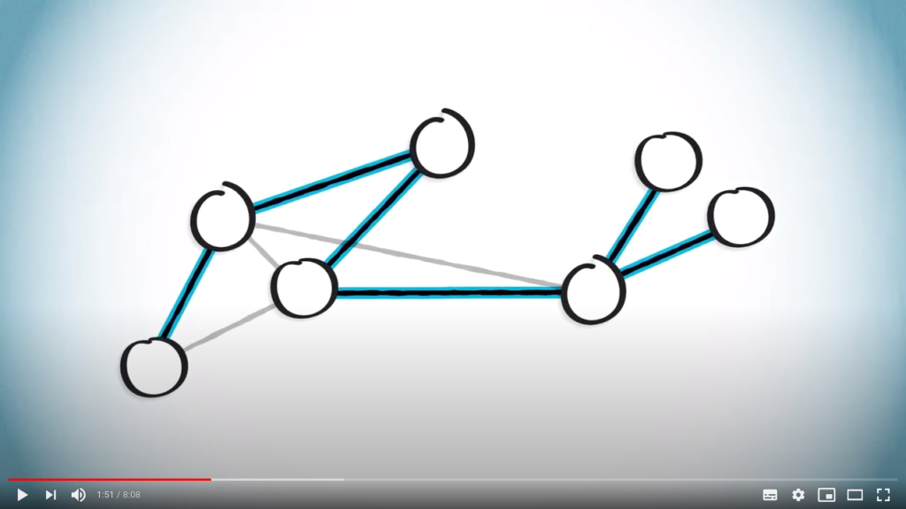
Now, a spanning tree of a graph is a tree obtained from by removing some edges. To illustrate, consider the following graph. We can obtain a spanning tree by keeping only the following edges.
Note that for a given graph, other spanning trees can be defined, such as this one.
Finding spanning trees can have many applications. In particular, finding a spanning tree is very useful when you want to avoid loops, such as in routing algorithms in networking.
Another example of its usefulness is when assessing if a graph is connected. Imagine that you want to isolate a portion of a highway for maintenance. First, you need to make sure that the graph of streets remain connected during the constructions work.
In this lesson, we’re going to see how to find a path between two vertices of a connected graph, so that we’re able to navigate between any two points.
By definition, a spanning tree will include exactly one path between those two points.
We will compare two approaches: the depth-first search and the breadth-first search.
Depth-first search
The main idea of a depth-first search is to keep exploring the graph, jumping from a given vertex to one of its unexplored neighbors. Sometimes, all neighbors of the vertex we’re in have already been explored, in which case we turn back, following the trail in the opposite direction until we find an unexplored vertex to jump to.
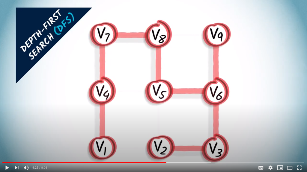
Take the following example. A depth-first search, or DFS, can be performed in the following way. Let’s start from .
First we go up. Note that we could have chosen to go right.
We continue exploring the graph, we go up again.
Next, we have only one unexplored neighbor, which is on the right. So we go right.
Now we go down. Alternatively, we could have continued right.
From here, there are four neighbors, two of which are unexplored. We choose to go right.
Next, we go up.
At this point, we can’t go further, because all the current neighbors have already been explored. We go back to the last vertex for which there was an unexplored neighbor, which is the previous one.
And we go down.
From this vertex, there’s only one remaining, unexplored neighbor, which is the one on the left. This is the last unexplored vertex in the graph.
The graph in red is a spanning tree obtained from the graph using a DFS.
DFS is a simple yet efficient strategy to ensure that all accessible vertices are explored.
It is an easy way to find the exit of a maze, or to make sure streets remain connected during construction work.
However, it doesn’t necessarily yield shortest paths between pairs of vertices in the graph. In this example, it takes 7 hops to travel from to , despite the fact that these could be linked with just 1 hop.
Breadth-first search
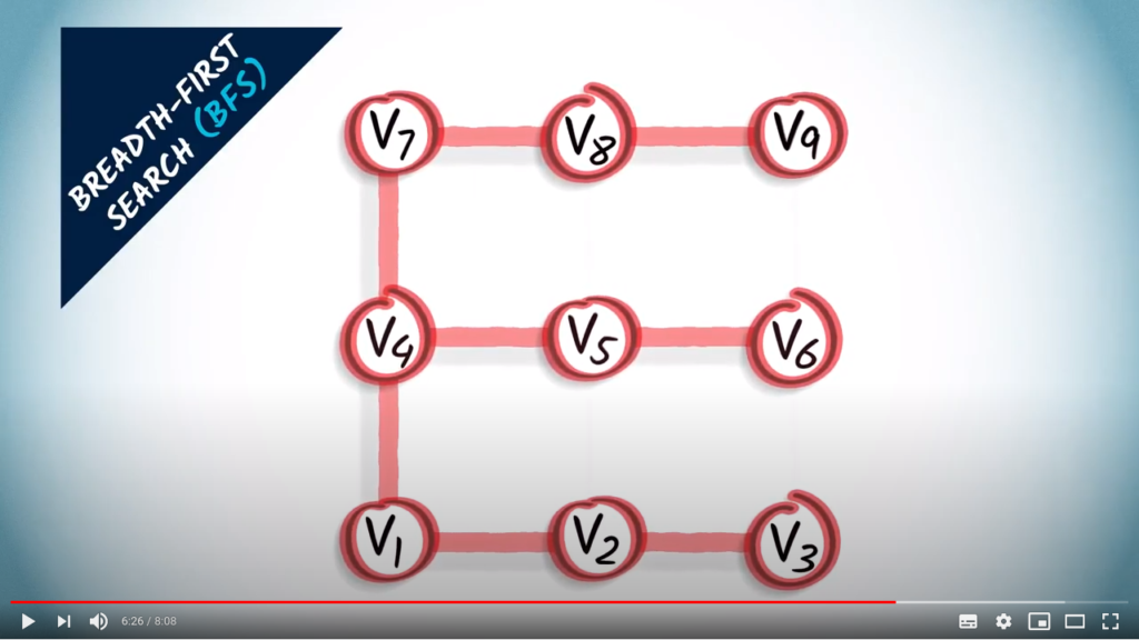
The other approach I will describe here is the breadth-first search. When using a breadth-first search, or BFS, we explore the graph by gradually increasing the number of hops from the initial vertex.
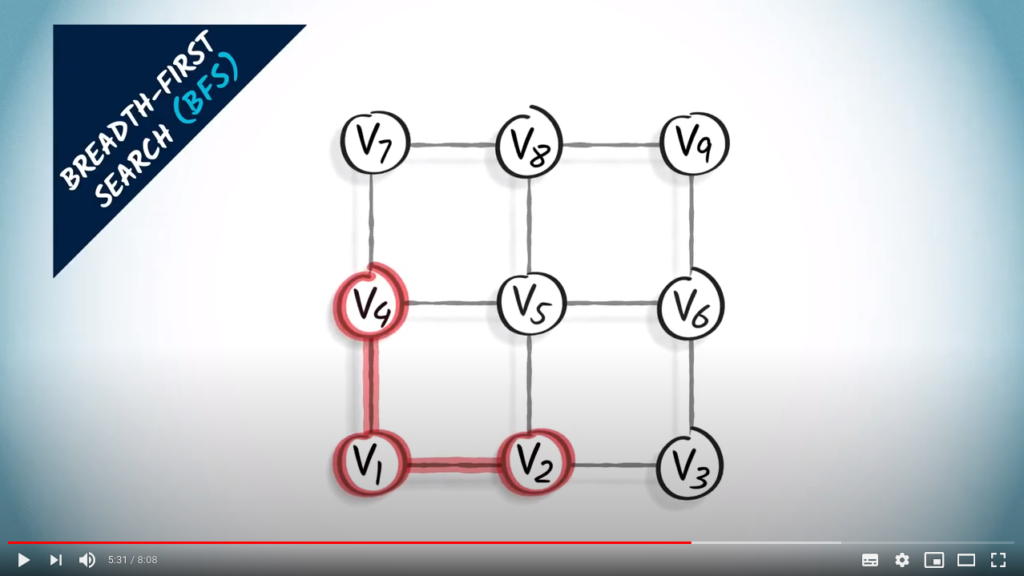
Let’s consider the same example, where we start in .
We start by exploring all vertices one hop away from : we thus connect both and to .
Then we explore all vertices two hops away from . A vertex two hops away from is one hop away from a vertex that’s one hop away from . So we look at the neighbors of and and connect them to or . We obtain , and .
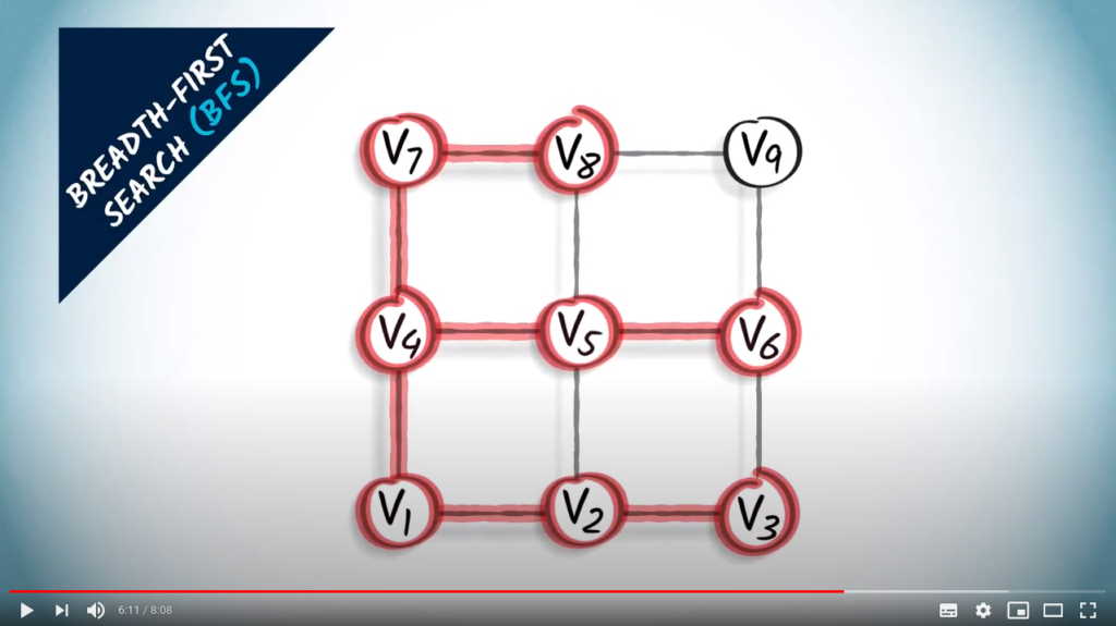
Then we explore the vertices three hops away from vertex . So we look at vertices two hops away, which are , and , and at their unexplored neighbors. We obtain and .
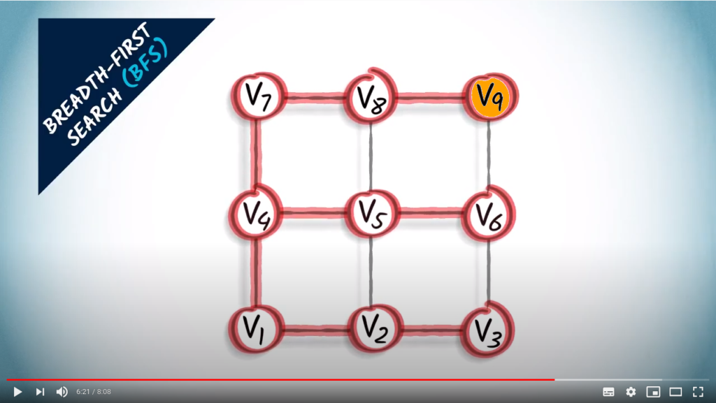
Finally, the orange vertex is one hop away from , which is three hops away from vertex . We connect them.
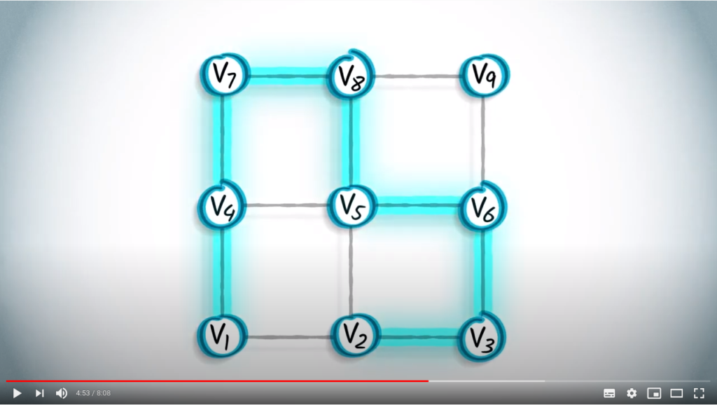
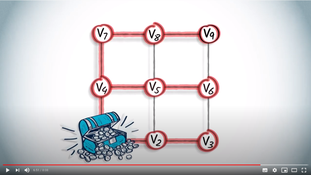
The resulting graph in red is a spanning tree obtained from the BFS, which is made exclusively of shortest paths from vertex to the other vertices of the graph.
A BFS is a cautious strategy in which we try to keep the distances to the initial vertex as small as possible during exploration.
This is especially useful when the initial vertex contains specific resources that we might need at any moment. However, it does require more organization than its simpler DFS counterpart.
Comparison between BFS and DFS
In the previous example, the spanning trees obtained by a BFS and a DFS are very different.
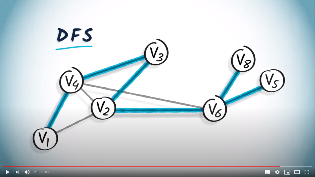
Here’s another example using the graph we considered earlier in this lesson.
This is a spanning tree obtained from a DFS starting from .
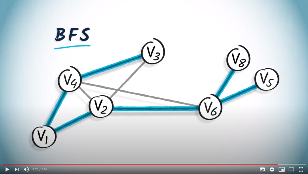
While this is a spanning tree obtained from a BFS starting from .
Because a BFS is performed by gradually increasing the hops from , a spanning tree obtained from a BFS will always provide the shortest path from to any other vertex in the graph, provided that the graph is unweighted. This can be seen clearly in this example.
Concluding words
In the next lesson, we will see how the difference between a BFS and a DFS directly relates to the type of memory structure that can be used to implement these two algorithms.
Properties of the BFS
In order to understand this section properly, you should first study the proposed implementation of the BFS here.
When writing an algorithm, it is important to answer three questions:
Will it terminate?
Is it correct?
How complex is it?
Termination
The algorithm only visits once each vertex that can be attained. Since the number of vertices is finite, the algorithm will eventually terminate.
Correctness
We want to show that the BFS algorithm returns a shortest path from a vertex to all other vertices that can be attained from through graph edges.
We are going to show that:
All vertices are visited in increasing distance to .
Obtained paths are of minimum length.
All attainable vertices are visited.
All vertices are visited in increasing distance to u
Let’s assume by the contradiction the first moment when a vertex is added to the FIFO, and there already exists a vertex inside it such that .
Let’s note the vertex, neighbor of , that adds to the FIFO. There can be two cases:
Either is closer to than and we reach a contradiction. Indeed, when was added, there was a vertex in the FIFO that was already farther. Therefore, this is not the first moment when this situation happens.
Or the distance from to is the same as the one from to . We therefore conclude that is closer from than . Let be a predecessor of on a shortest path from to . has not been visited, otherwise would have added it to the FIFO. By recurrence, we see that a direct neighbor of hasn’t been added to the FIFO, thus . cannot thus be closer from than .
Obtained paths are of minimum length
The proof is performed by induction. We will show that, at any moment, all paths in the FIFO are of minimal length.
This is trivially true for starting vertex , as it is at distance 0 from itself.
As shown previously, all vertices are visited in increasing distance to . This ensures that adding a vertex to the FIFO is always performed by a neighbor that is a predecessor along a shortest path initiated from .
All attainable vertices are visited
By contradiction, let be an attainable vertex, but not yet visited, at minimal distance from . Let us consider a shortest path from to . Let be the predecessor of along that path.
Thus, has not been visited, otherwise it would have been added to the FIFO. Therefore, is attainable and not yet visited, and is closer from than . We reach a contradiction.
Complexity
The algorithm only visits once each vertex, and checks the list of unprocessed neighbors each time. Therefore, its complexity is , where is the number of edges in the graph and is the number of vertices.
Properties of the DFS
Termination
The algorithm only visits once each vertex that can be attained. Since the number of vertices is finite, the algorithm will eventually terminate.
Correctness
We want to show that the algorithm is such that it will visit all the vertices attainable from .
To verify this property, we first remark that all the visited vertices during a DFS are indeed attainable. This can easily be shown by induction ( is trivially attainable from itself, then neighboring vertices are also attainable).
Then, we have to verify that all attainable vertices are visited by the DFS. Let’s proceed by contradiction. A vertex which is attainable is, by definition, such that there exists a path from to in the graph. On such a path, we consider the vertex just before . This vertex cannot be visited, otherwise would have been visited. By induction, we conclude that has not been visited, and reach a contradiction.
Complexity
The algorithm only visits once each vertex, and checks the list of unprocessed neighbors each time. Therefore, its complexity is , where is the number of edges in the graph and is the number of vertices.
To go further
Beam search: a variation of the BFS to accelerate it while sacrificing the guarantee it will find the shortest path.
IDDFS: a mixed approach between DFS and BFS that takes the best of both worlds.


 composed of a set of vertices
  and a set of edges
  . Now we need to define a few more things.
 is in
is in 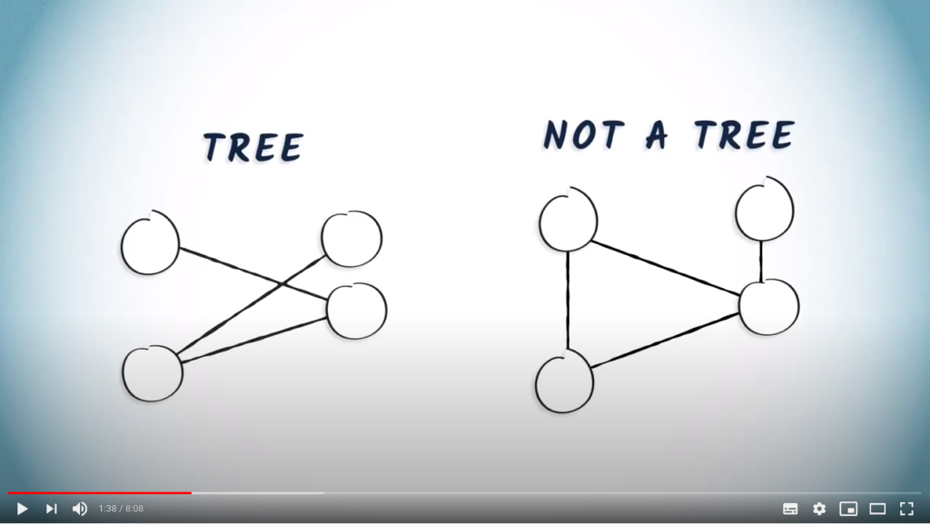


 .
.


 to
to  , despite the fact that these could be linked with just 1 hop.
 and
and  to
to 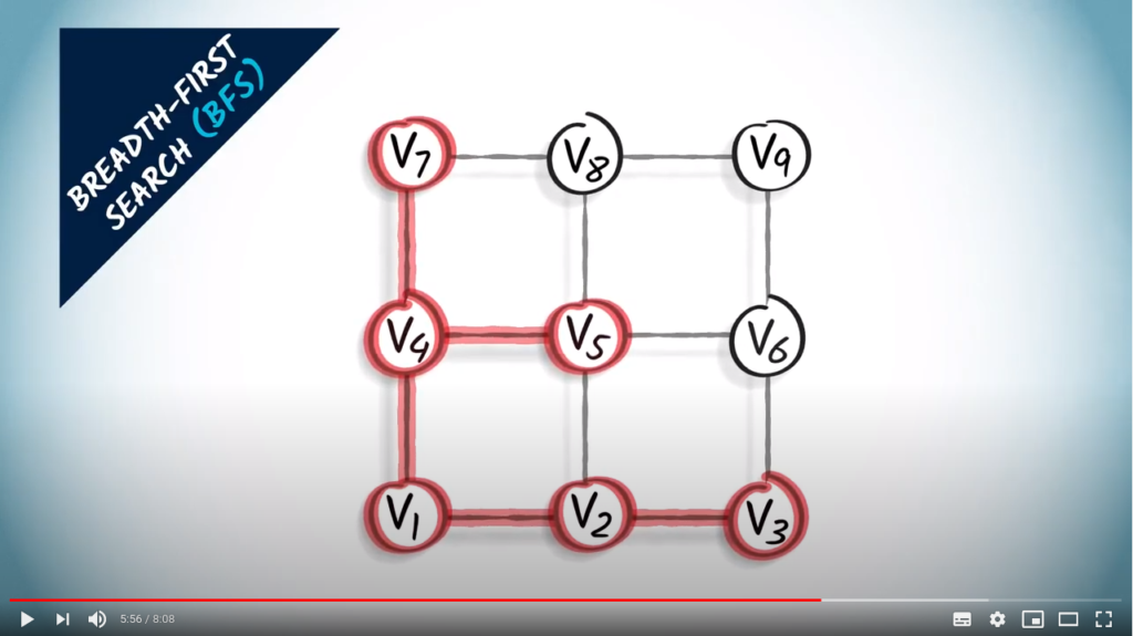
 ,
,  and
and  .
.
 and
and  .
.
 to all other vertices that can be attained from
  is added to the FIFO, and there already exists a vertex
  inside it such that
  .
. the vertex, neighbor of
  be a predecessor of
  .
.  , where
  is the number of edges in the graph and
  is the number of vertices.