Approximate solutions

Example: coloring graphs

The exact algorithm

Let us consider the following example: we call coloring of a graph a vector of integers, each associated with one of its vertices. These integers are called vertex colors, and can be identical.

A coloring is said to be clean if all vertices connected by an edge are of different colors. The chromatic number of a graph is the minimum number of colors that appear in a specific coloring.

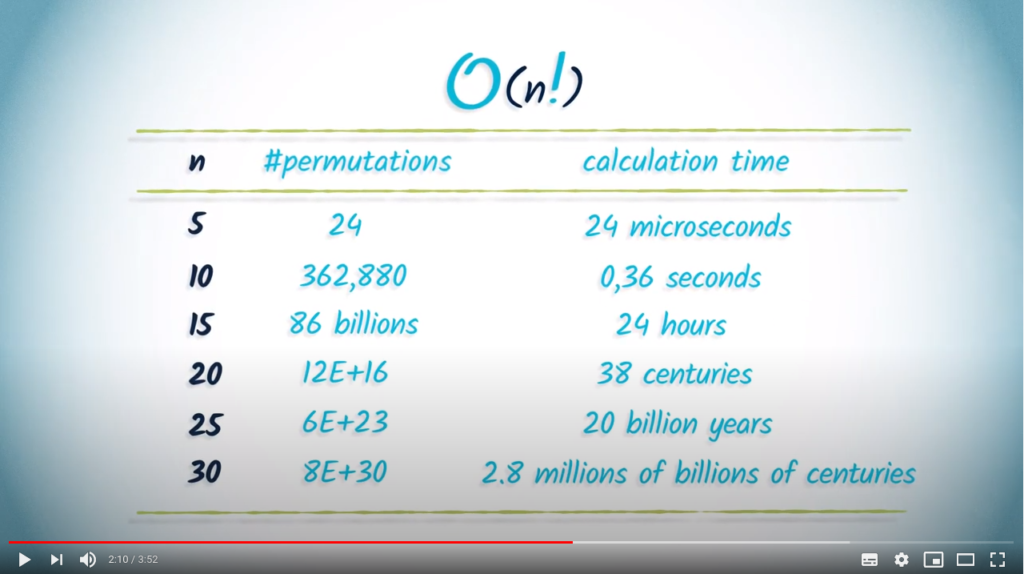
This problem is a known example of a NP-Complete problem. One way to solve it accurately is to list all possible 1-color colorings, then 2-colors, etc. until you find a clean coloring.

The following Python code solves the problem as described above:

# Easy iteration over permutations
import itertools



# Function to check if a coloring is correct
# A coloring is correct if no neighbors share a color
def check_coloring (graph, colors) :
    for vertex in range(len(graph)) : 
        for neighbor in graph[vertex] :
            if colors[vertex] == colors[neighbor] :
                return False
    return True



# This function returns a coloring of the given graph using a minimum number of colors
def find_coloring (graph) :
    
    # We gradually increase the number of available colors
    for nb_colors in range(len(graph)) :
        
        # We test all possible arrangements of colors
        # This could be improved as product(2, ...)  is a subset of product(3, ...) for instance
        for coloring in itertools.product(range(nb_colors), repeat=len(graph)) :
            print("Nb colors :", nb_colors, "- Candidate coloring :", coloring)
            if check_coloring(graph, coloring) :
                return coloring

    
    
# Test graph
graph = [[1, 2, 5], [0, 2, 5], [0, 1], [4, 5], [3, 5], [0, 1, 3, 4]]
result = find_coloring(graph)
print(result)

In that example, a graph is implemented in the form of a list of lists. It contains 6 vertices, and 8 (symetric) edges. The solution returned by the algorithm is:

[0, 1, 2, 0, 1, 2]

This indicates that three colors are sufficient to have a clean coloring of the graph, with and sharing color 0, and sharing color 1, and and sharing color 2.

The greedy approach

This algorithm is very complex and a well-known approximate solution is to sort the vertices by decreasing number of neighbors, coloring them in this order by choosing the smallest positive color that leaves the coloring clean. This approximate algorithm is described below:

# For min-heaps
import heapq



# Function to check if a coloring is correct
# A coloring is correct if no neighbours share a color
def check_coloring (graph, colors) :
    for vertex in range(len(graph)) :
        if colors[vertex] is not None :
            for neighbor in graph[vertex] :
                if colors[neighbor] is not None :
                    if colors[vertex] == colors[neighbor] :
                        return False
    return True
    
    
 
# This function greedily tries to color the graph from highest degree node to lowest degree one
def greedy_coloring (graph) :
    
    # Sorting nodes in descending degree order using a max-heap (negative min-heap)
    heap = []
    for vertex in range(len(graph)) :
        heapq.heappush(heap, (-len(graph[vertex]), vertex))
    
    # Coloring
    colors = [None] * len(graph)
    while len(heap) > 0 :
        degree, vertex = heapq.heappop(heap)
        for color in range(len(graph)) :
            colors[vertex] = color
            if check_coloring(graph, colors) :
                break
    return colors
    
    
    
# Test graph
graph = [[1, 2, 5], [0, 2, 5], [0, 1], [4, 5], [3, 5], [0, 1, 3, 4]]
result = greedy_coloring(graph)
print(result)

This algorithm is much less complex than the previous one, and therefore allows considering graphs with a lot more vertices.

Here, we obtain the following result:

[0, 1, 2, 0, 1, 2]

Note that here, we find the same result as the exhaustive algorithm. However this may not be always the case.

Simulations

In order to evaluate the quality of our approximate algorithm, we will focus on two things: computation time and accuracy. To test these two quantities, we will average results on a large number of random graphs.

The following program, measure_greedy.py, returns the average execution time of the greedy approach for solving the considered problem, as well as the average number of colors needed for a fixed-size graph:

# Various imports
import math
import random
import heapq
import time
import sys



# Arguments
NB_NODES = int(sys.argv[1])
EDGE_PROBABILITY = math.log(NB_NODES) / NB_NODES
NB_TESTS = int(sys.argv[2])



# Set a fixed random seed for comparing scripts on same graphs
random.seed(NB_NODES)



# Generates an Erdos-Renyi random graph
def generate_graph () :
    graph = [[] for i in range(NB_NODES)]
    for i in range(NB_NODES) :
        for j in range(i + 1, NB_NODES) :
            if random.random() < EDGE_PROBABILITY :
                graph[i].append(j)
                graph[j].append(i)
    return graph



# Function to check if a coloring is correct
# A coloring is correct if no neighbors share a color
def check_coloring (graph, colors) :
    for vertex in range(len(graph)) :
        if colors[vertex] is not None :
            for neighbor in graph[vertex] :
                if colors[neighbor] is not None :
                    if colors[vertex] == colors[neighbor] :
                        return False
    return True
    
    
 
# This function greedily tries to color the graph from highest degree node to lowest degree one
def greedy_coloring (graph) :
    
    # Sorting nodes in descending degree order using a max-heap (negative min-heap)
    heap = []
    for vertex in range(len(graph)) :
        heapq.heappush(heap, (-len(graph[vertex]), vertex))
    
    # Coloring
    colors = [None] * len(graph)
    while len(heap) > 0 :
        degree, vertex = heapq.heappop(heap)
        for color in range(len(graph)) :
            colors[vertex] = color
            if check_coloring(graph, colors) :
                break
    return colors



# Tests
average_time = 0.0
average_solution_length = 0.0
for i in range(NB_TESTS) :
    graph = generate_graph()
    time_start = time.time()
    solution = greedy_coloring(graph)
    average_solution_length += len(set(solution)) / NB_TESTS
    average_time += (time.time() - time_start) / NB_TESTS



# Print average time as a function of problem size
print(NB_NODES, ",", average_time, ",", average_solution_length)

Similarly, the following program measure_exhaustive.py evaluates the exhaustive solution:

# Various imports
import math
import random
import time
import sys
import itertools



# Arguments
NB_NODES = int(sys.argv[1])
EDGE_PROBABILITY = math.log(NB_NODES) / NB_NODES
NB_TESTS = int(sys.argv[2])



# Set a fixed random seed for comparing scripts on same graphs
random.seed(NB_NODES)



# Generates an Erdos-Renyi random graph
def generate_graph () :
    graph = [[] for i in range(NB_NODES)]
    for i in range(NB_NODES) :
        for j in range(i + 1, NB_NODES) :
            if random.random() < EDGE_PROBABILITY :
                graph[i].append(j)
                graph[j].append(i)
    return graph




# Function to check if a coloring is correct
# A coloring is correct if no neighbors share a color
def check_coloring (graph, colors) :
    for vertex in range(len(graph)) : 
        for neighbor in graph[vertex] :
            if colors[vertex] == colors[neighbor] :
                return False
    return True



# This function returns a coloring of the given graph using a minimum number of colors
def find_coloring (graph) :
    
    # We gradually increase the number of available colors
    for nb_colors in range(len(graph)) :
        
        # We test all possible arrangements of colors
        # This could be improved as product(2, ...)  is a subset of product(3, ...) for instance
        for coloring in itertools.product(range(nb_colors), repeat=len(graph)) :
            if check_coloring(graph, coloring) :
                return coloring



# Tests
average_time = 0.0
average_solution_length = 0.0
for i in range(NB_TESTS) :
    graph = generate_graph()
    time_start = time.time()
    solution = find_coloring(graph)
    average_solution_length += len(set(solution)) / NB_TESTS
    average_time += (time.time() - time_start) / NB_TESTS



# Print average time as a function of problem size
print(NB_NODES, ",", average_time, ",", average_solution_length)

Making curves

In order to automatize things a bit, we will adapt our code to take argument out of the command line and output a processable file:

We can now run the following commands to run both algorithms on random graphs (100 graphs per graph order). The exhaustive search will only be evaluated on a subset of the graph orders due to time considerations:

for n in {5..100}; do python measure_greedy.py {n} 100 >> results_exhaustive.csv ; done

Let’s compare execution times using Libreoffice:

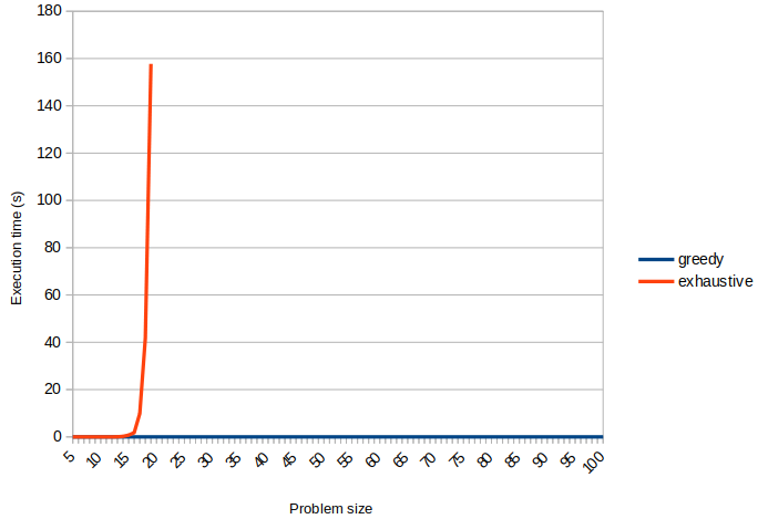
Clearly, the gain in execution time is significant. Similarly, let us compare the average chromatic numbers found for the two algorithms:

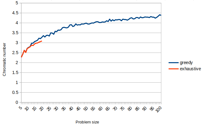
Looking at the precision curve, it seems that the precision loss is not very high, at least for the problem sizes that could be computed using the exhaustive approach. For larger graphs, we cannot compute the exact solution due to complexity of finding it.

In order to evaluate a bit more that aspect, we are going to evaluate the solutions found using the greedy approach on bipartite graphs, for which we know the chromatic number is always 2:

# Generates a bipartite Erdos-Renyi random graph
def generate_graph () :
    graph = [[] for i in range(NB_NODES)]
    for i in range(NB_NODES) :
        for j in range(i + 1, NB_NODES) :
            if i % 2 != j % 2 and random.random() < EDGE_PROBABILITY :
                graph[i].append(j)
                graph[j].append(i)
    return graph

We obtain the following results:

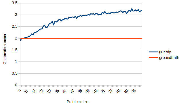
Here again, the result seems reasonable, which leads us think this heuristic is well-suited to the problem.

You should still note that for low problem sizes, the chromatic number found is sometimes lower than 2, which seems wrong. However, notice that the random graph generator does not check connectivity of the graph, which may lead to disconnected graphs for low vertex counts.